>吴恩达机器学习课程链接
>课程总结和笔记链接
实验二的原始代码和使用数据可至课程链接-课时60-章节8编程作业中下载包括逻辑回归的损失函数、梯度、自动优化、预测以及正则化后的损失函数、梯度等
环境——Matlab R2018b/Octave
一般Logistic Regression
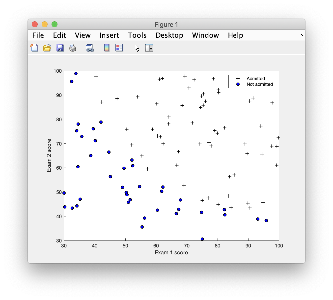
Part 1: Plotting
plotData.m
二分类,在图上用不同的标记表示两类数据1
2
3
4
5
6
7
8
9
10
11
12
13
14
15
16
17
18
19
20
21
22
23
24
25function plotData(X, y)
%PLOTDATA Plots the data points X and y into a new figure
% PLOTDATA(x,y) plots the data points with + for the positive examples
% and o for the negative examples. X is assumed to be a Mx2 matrix.
% Create New Figure
figure; hold on;
% ====================== YOUR CODE HERE ======================
% Instructions: Plot the positive and negative examples on a
% 2D plot, using the option 'k+' for the positive
% examples and 'ko' for the negative examples.
%
positive = find(y == 1);
negative = find(y == 0);
plot(X(positive, 1), X(positive, 2), 'k+')
plot(X(negative, 1), X(negative, 2), 'ko', 'MarkerFaceColor', 'b')
% =========================================================================
hold off;
end
运行结果
Part 2: Compute Cost and Gradient
sigmoid.m1
2
3
4
5
6
7
8
9
10
11
12
13
14
15
16function g = sigmoid(z)
%SIGMOID Compute sigmoid function
% g = SIGMOID(z) computes the sigmoid of z.
% You need to return the following variables correctly
g = zeros(size(z));
% ====================== YOUR CODE HERE ======================
% Instructions: Compute the sigmoid of each value of z (z can be a matrix,
% vector or scalar).
g = 1 ./ (exp(-z)+1);
% =============================================================
end
costFunction.m1
2
3
4
5
6
7
8
9
10
11
12
13
14
15
16
17
18
19
20
21
22
23
24
25
26
27
28
29
30
31
32
33
34
35
36
37
38
39function [J, grad] = costFunction(theta, X, y)
%COSTFUNCTION Compute cost and gradient for logistic regression
% J = COSTFUNCTION(theta, X, y) computes the cost of using theta as the
% parameter for logistic regression and the gradient of the cost
% w.r.t. to the parameters.
% Initialize some useful values
m = length(y); % number of training examples
% You need to return the following variables correctly
J = 0;
grad = zeros(size(theta));
alpha = 0.01;
% ====================== YOUR CODE HERE ======================
% Instructions: Compute the cost of a particular choice of theta.
% You should set J to the cost.
% Compute the partial derivatives and set grad to the partial
% derivatives of the cost w.r.t. each parameter in theta
%
% Note: grad should have the same dimensions as theta
%
pos = y == 1;
neg = y == 0;
h_pos = sigmoid(X(pos, :) * theta);
J_pos = sum(-log(h_pos));
h_neg = sigmoid(X(neg, :) * theta);
J_neg = sum(-log(1 - h_neg));
J = (J_pos + J_neg)/m;
grad = (sum(X .* (sigmoid(X * theta) - y)))' * alpha;
% =============================================================
end
运行结果
Cost at initial theta (zeros): 0.693147
Expected cost (approx): 0.693
Gradient at initial theta (zeros):
 -0.100000
 -12.009217
 -11.262842
Expected gradients (approx):
 -0.1000
 -12.0092
 -11.2628

Cost at test theta: 0.218330
Expected cost (approx): 0.218
Gradient at test theta:
 0.042903
 2.566234
 2.646797
Expected gradients (approx):
 0.043
 2.566
 2.647

Program paused. Press enter to continue.
Part 3: Optimizing using fminunc
plotDecisionBoundary.m
画出决策边界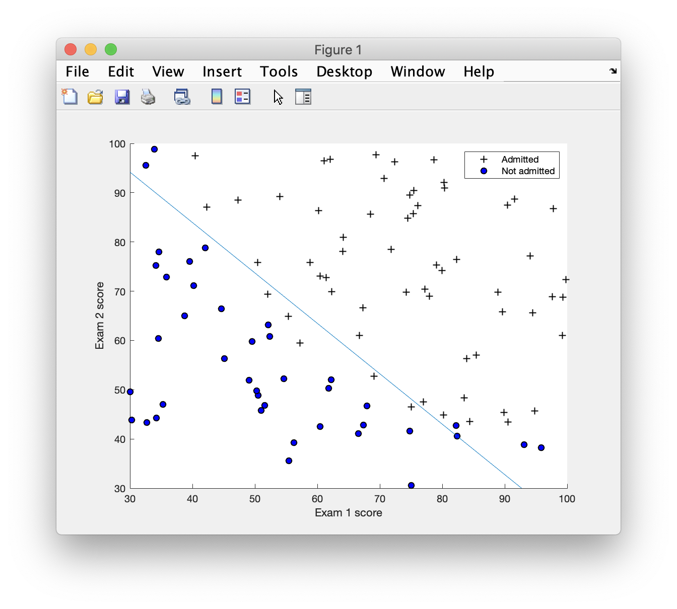
使用自动寻找最优参数函数(代码在主函数中)1
2[theta, cost] = ...
fminunc(@(t)(costFunction(t, X, y)), initial_theta, options);
运行结果
Cost at theta found by fminunc: 0.203498
Expected cost (approx): 0.203
theta:
 -25.161343
 0.206232
 0.201472
Expected theta (approx):
 -25.161
 0.206
 0.201
Part 4: Predict and Accuracies
预测一个实例&&查看模型在训练集上的准确率
predict.m1
2
3
4
5
6
7
8
9
10
11
12
13
14
15
16
17
18
19
20
21
22function p = predict(theta, X)
%PREDICT Predict whether the label is 0 or 1 using learned logistic
%regression parameters theta
% p = PREDICT(theta, X) computes the predictions for X using a
% threshold at 0.5 (i.e., if sigmoid(theta'*x) >= 0.5, predict 1)
m = size(X, 1); % Number of training examples
% You need to return the following variables correctly
p = zeros(m, 1);
% ====================== YOUR CODE HERE ======================
% Instructions: Complete the following code to make predictions using
% your learned logistic regression parameters.
% You should set p to a vector of 0's and 1's
%
p = floor(sigmoid(X * theta) / 0.5);
% =========================================================================
end
运行结果
For a student with scores 45 and 85, we predict an admission probability of 0.776291
Expected value: 0.775 +/- 0.002

Train Accuracy: 89.000000
Expected accuracy (approx): 89.0
主函数代码
1 | %% Machine Learning Online Class - Exercise 2: Logistic Regression |
正则化
Part 1: Regularized Logistic Regression
costFunctionReg.m
加入正则化项的代价函数和梯度1
2
3
4
5
6
7
8
9
10
11
12
13
14
15
16
17
18
19
20
21
22
23
24
25
26
27
28
29
30
31
32
33
34
35
36
37function [J, grad] = costFunctionReg(theta, X, y, lambda)
%COSTFUNCTIONREG Compute cost and gradient for logistic regression with regularization
% J = COSTFUNCTIONREG(theta, X, y, lambda) computes the cost of using
% theta as the parameter for regularized logistic regression and the
% gradient of the cost w.r.t. to the parameters.
% Initialize some useful values
m = length(y); % number of training examples
% You need to return the following variables correctly
J = 0;
grad = zeros(size(theta));
% ====================== YOUR CODE HERE ======================
% Instructions: Compute the cost of a particular choice of theta.
% You should set J to the cost.
% Compute the partial derivatives and set grad to the partial
% derivatives of the cost w.r.t. each parameter in theta
pos = y == 1;
neg = y == 0;
h_pos = sigmoid(X(pos, :) * theta);
J_pos = sum(-log(h_pos));
h_neg = sigmoid(X(neg, :) * theta);
J_neg = sum(-log(1 - h_neg));
J_reg = lambda/2 * sum(theta(2:end, :) .^ 2);
J = (J_pos + J_neg + J_reg)/m;
grad = (sum(X .* (sigmoid(X * theta) - y)))' / m;
grad_reg = ((lambda * theta(2:end, :)) / m);
grad(2:end, :) = grad(2:end, :) + grad_reg;
% =============================================================
end
运行结果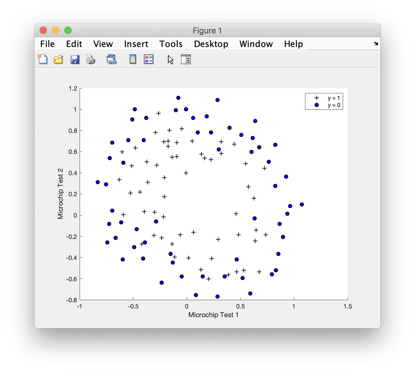
Cost at initial theta (zeros): 0.693147
Expected cost (approx): 0.693
Gradient at initial theta (zeros) - first five values only:
 0.008475
 0.018788
 0.000078
 0.050345
 0.011501
Expected gradients (approx) - first five values only:
 0.0085
 0.0188
 0.0001
 0.0503
 0.0115

Program paused. Press enter to continue.

Cost at test theta (with lambda = 10): 3.164509
Expected cost (approx): 3.16
Gradient at test theta - first five values only:
 0.346045
 0.161352
 0.194796
 0.226863
 0.092186
Expected gradients (approx) - first five values only:
 0.3460
 0.1614
 0.1948
 0.2269
 0.0922

Program paused. Press enter to continue.
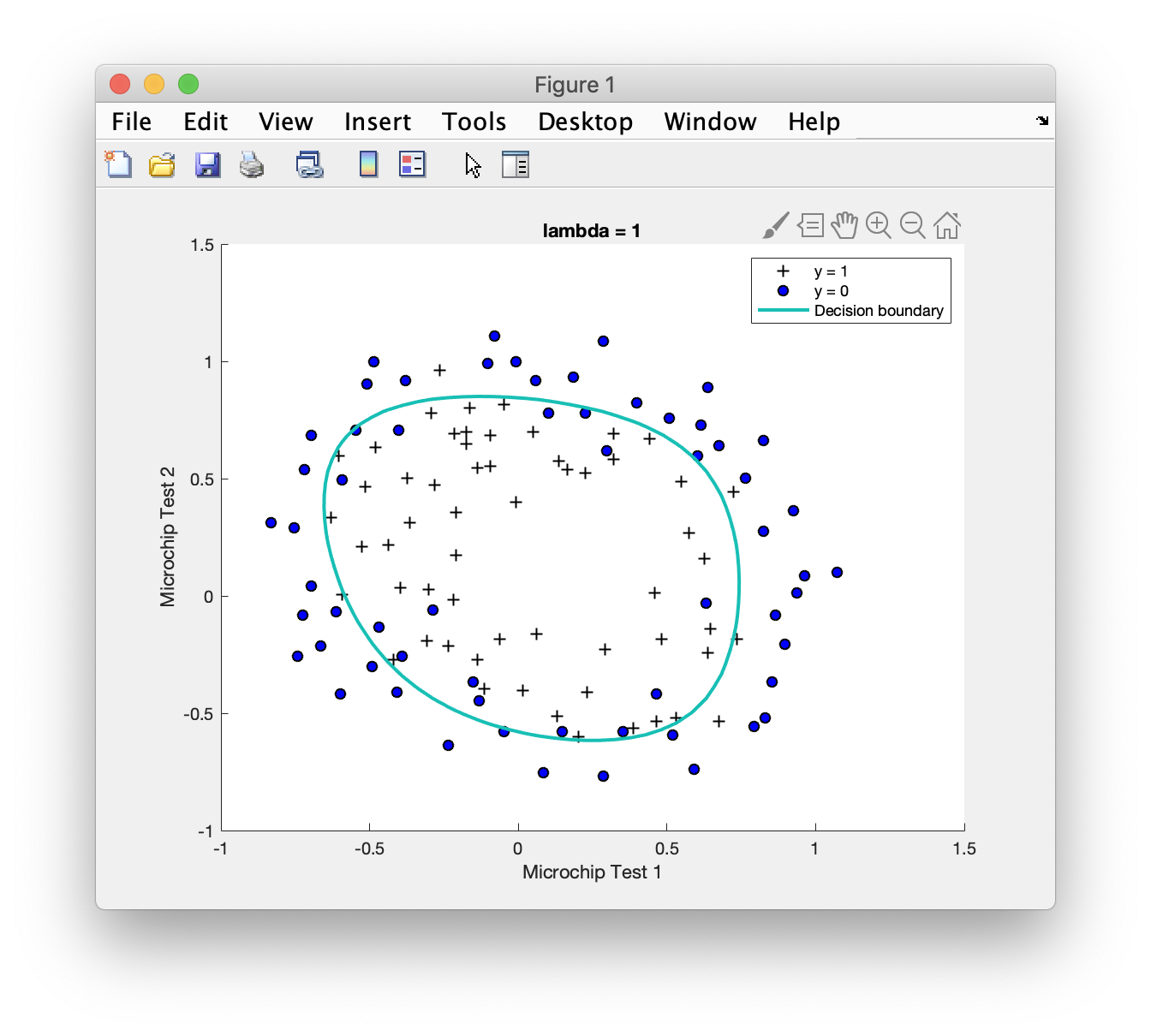
Part 2: Regularization and Accuracies
运行结果
Train Accuracy: 83.050847
Expected accuracy (with lambda = 1): 83.1 (approx)
主函数代码
1 | %% Machine Learning Online Class - Exercise 2: Logistic Regression |
实验二完成