>吴恩达机器学习课程链接
>课程总结和笔记链接
实验一的原始代码和使用数据可至课程链接-课时45-章节6编程作业中下载包括热身练习、单变量/多变量的损失函数计算、梯度下降的参数更新、特征归一化、正规方程等
环境——Matlab R2018b/Octave
单特征
Part 1: Basic Function
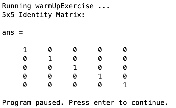
输出一个5X5单位矩阵
warmUpExercise.m1
2
3
4
5
6
7
8
9
10
11
12
13
14
15function A = warmUpExercise()
%WARMUPEXERCISE Example function in octave
% A = WARMUPEXERCISE() is an example function that returns the 5x5 identity matrix
A = [];
% ============= YOUR CODE HERE ==============
% Instructions: Return the 5x5 identity matrix
% In octave, we return values by defining which variables
% represent the return values (at the top of the file)
% and then set them accordingly.
A = eye(5);
% ===========================================
end
运行结果
Part 2: Plotting
显示数据集ex1data1.txt
plotData.m1
2
3
4
5
6
7
8
9
10
11
12
13
14
15
16
17
18
19
20
21
22
23function plotData(x, y)
%PLOTDATA Plots the data points x and y into a new figure
% PLOTDATA(x,y) plots the data points and gives the figure axes labels of
% population and profit.
figure; % open a new figure window
% ====================== YOUR CODE HERE ======================
% Instructions: Plot the training data into a figure using the
% "figure" and "plot" commands. Set the axes labels using
% the "xlabel" and "ylabel" commands. Assume the
% population and revenue data have been passed in
% as the x and y arguments of this function.
%
% Hint: You can use the 'rx' option with plot to have the markers
% appear as red crosses. Furthermore, you can make the
% markers larger by using plot(..., 'rx', 'MarkerSize', 10);
plot(x, y, 'rx', 'MarkerSize', 10);
xlabel('population');
ylabel('revenue');
% ============================================================
end
运行结果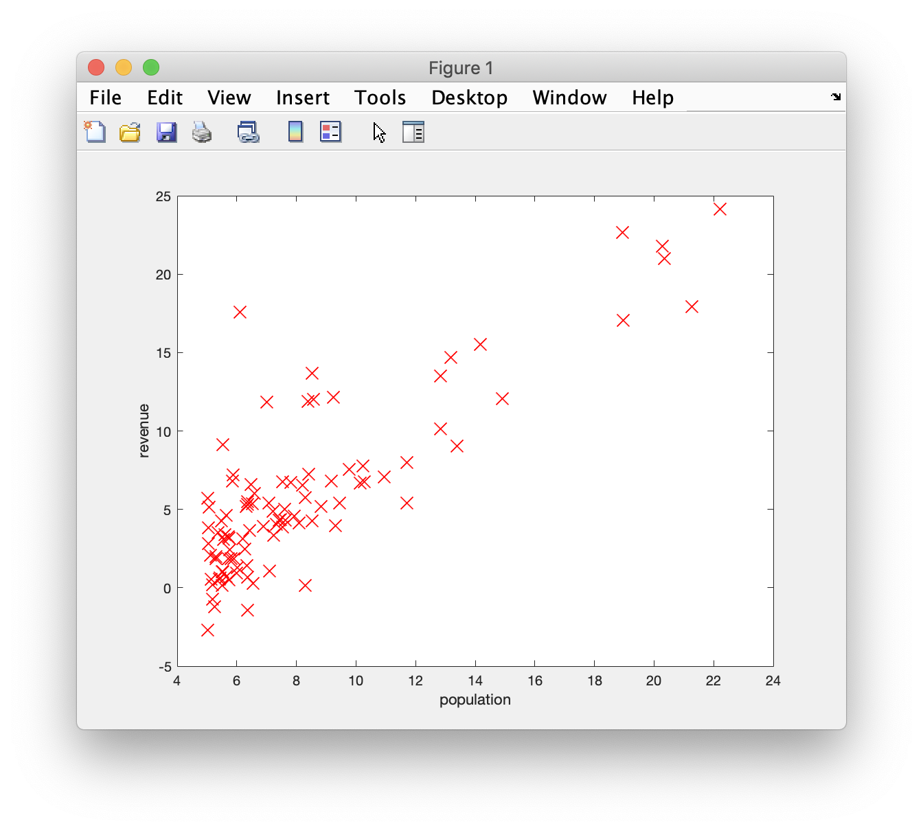
Part 3: Cost and Gradient descent
损失函数和梯度下降
computeCost.m1
2
3
4
5
6
7
8
9
10
11
12
13
14
15
16
17
18
19
20
21function J = computeCost(X, y, theta)
%COMPUTECOST Compute cost for linear regression
% J = COMPUTECOST(X, y, theta) computes the cost of using theta as the
% parameter for linear regression to fit the data points in X and y
% Initialize some useful values
m = length(y); % number of training examples
% You need to return the following variables correctly
J = 0;
% ====================== YOUR CODE HERE ======================
% Instructions: Compute the cost of a particular choice of theta
% You should set J to the cost.
predictions = X * theta;
sqrErrors = (predictions - y).^2;
J = 1 / (2 * m) * sum(sqrErrors);
% =========================================================================
end
gradientDescent.m1
2
3
4
5
6
7
8
9
10
11
12
13
14
15
16
17
18
19
20
21
22
23
24
25
26
27
28
29
30
31function [theta, J_history] = gradientDescent(X, y, theta, alpha, num_iters)
%GRADIENTDESCENT Performs gradient descent to learn theta
% theta = GRADIENTDESCENT(X, y, theta, alpha, num_iters) updates theta by
% taking num_iters gradient steps with learning rate alpha
% Initialize some useful values
m = length(y); % number of training examples
J_history = zeros(num_iters, 1);
for iter = 1:num_iters
% ====================== YOUR CODE HERE ======================
% Instructions: Perform a single gradient step on the parameter vector
% theta.
%
% Hint: While debugging, it can be useful to print out the values
% of the cost function (computeCost) and gradient here.
%
predictions0 = 1 / m * sum(X * theta - y);
theta(1) = theta(1) - alpha * predictions0;
predictions1 = 1 / m * sum((X * theta - y) .* X(:,2));
theta(2) = theta(2) - alpha * predictions1;
% ============================================================
% Save the cost J in every iteration
J_history(iter) = computeCost(X, y, theta);
end
end
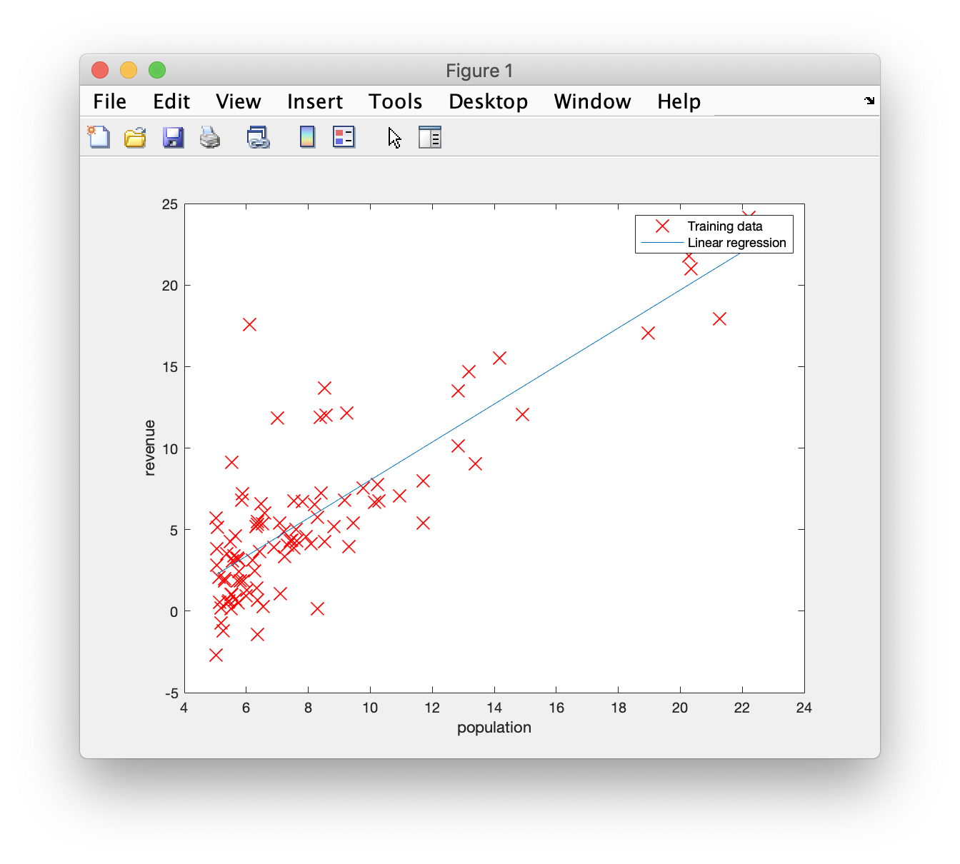
运行结果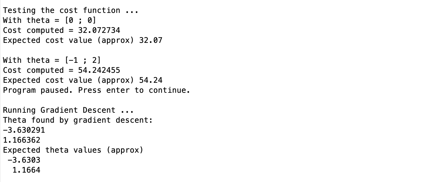
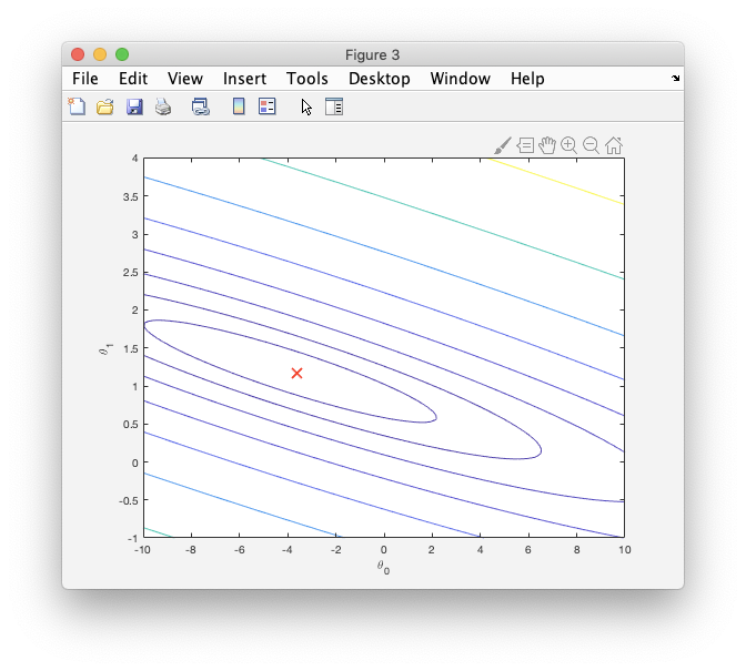
Part 4: Visualizing J(theta_0, theta_1)
参数更新视图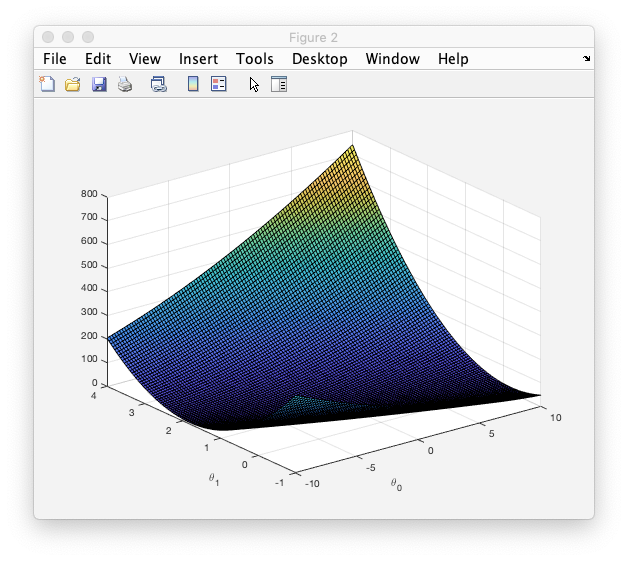
主函数代码
ex1.m1
2
3
4
5
6
7
8
9
10
11
12
13
14
15
16
17
18
19
20
21
22
23
24
25
26
27
28
29
30
31
32
33
34
35
36
37
38
39
40
41
42
43
44
45
46
47
48
49
50
51
52
53
54
55
56
57
58
59
60
61
62
63
64
65
66
67
68
69
70
71
72
73
74
75
76
77
78
79
80
81
82
83
84
85
86
87
88
89
90
91
92
93
94
95
96
97
98
99
100
101
102
103
104
105
106
107
108
109
110
111
112
113
114
115
116
117
118
119
120
121
122
123
124
125
126
127
128
129
130
131
132
133
134
135%% Machine Learning Online Class - Exercise 1: Linear Regression
% Instructions
% ------------
%
% This file contains code that helps you get started on the
% linear exercise. You will need to complete the following functions
% in this exericse:
%
% warmUpExercise.m
% plotData.m
% gradientDescent.m
% computeCost.m
% gradientDescentMulti.m
% computeCostMulti.m
% featureNormalize.m
% normalEqn.m
%
% For this exercise, you will not need to change any code in this file,
% or any other files other than those mentioned above.
%
% x refers to the population size in 10,000s
% y refers to the profit in $10,000s
%
%% Initialization
clear ; close all; clc
%% ==================== Part 1: Basic Function ====================
% Complete warmUpExercise.m
fprintf('Running warmUpExercise ... \n');
fprintf('5x5 Identity Matrix: \n');
warmUpExercise()
fprintf('Program paused. Press enter to continue.\n');
pause;
%% ======================= Part 2: Plotting =======================
fprintf('Plotting Data ...\n')
data = load('ex1data1.txt');
X = data(:, 1); y = data(:, 2);
m = length(y); % number of training examples
% Plot Data
% Note: You have to complete the code in plotData.m
plotData(X, y);
fprintf('Program paused. Press enter to continue.\n');
pause;
%% =================== Part 3: Cost and Gradient descent ===================
X = [ones(m, 1), data(:,1)]; % Add a column of ones to x
theta = zeros(2, 1); % initialize fitting parameters
% Some gradient descent settings
iterations = 1500;
alpha = 0.01;
fprintf('\nTesting the cost function ...\n')
% compute and display initial cost
J = computeCost(X, y, theta);
fprintf('With theta = [0 ; 0]\nCost computed = %f\n', J);
fprintf('Expected cost value (approx) 32.07\n');
% further testing of the cost function
J = computeCost(X, y, [-1 ; 2]);
fprintf('\nWith theta = [-1 ; 2]\nCost computed = %f\n', J);
fprintf('Expected cost value (approx) 54.24\n');
fprintf('Program paused. Press enter to continue.\n');
pause;
fprintf('\nRunning Gradient Descent ...\n')
% run gradient descent
theta = gradientDescent(X, y, theta, alpha, iterations);
% print theta to screen
fprintf('Theta found by gradient descent:\n');
fprintf('%f\n', theta);
fprintf('Expected theta values (approx)\n');
fprintf(' -3.6303\n 1.1664\n\n');
% Plot the linear fit
hold on; % keep previous plot visible
plot(X(:,2), X*theta, '-')
legend('Training data', 'Linear regression')
hold off % don't overlay any more plots on this figure
% Predict values for population sizes of 35,000 and 70,000
predict1 = [1, 3.5] *theta;
fprintf('For population = 35,000, we predict a profit of %f\n',...
predict1*10000);
predict2 = [1, 7] * theta;
fprintf('For population = 70,000, we predict a profit of %f\n',...
predict2*10000);
fprintf('Program paused. Press enter to continue.\n');
pause;
%% ============= Part 4: Visualizing J(theta_0, theta_1) =============
fprintf('Visualizing J(theta_0, theta_1) ...\n')
% Grid over which we will calculate J
theta0_vals = linspace(-10, 10, 100);
theta1_vals = linspace(-1, 4, 100);
% initialize J_vals to a matrix of 0's
J_vals = zeros(length(theta0_vals), length(theta1_vals));
% Fill out J_vals
for i = 1:length(theta0_vals)
for j = 1:length(theta1_vals)
t = [theta0_vals(i); theta1_vals(j)];
J_vals(i,j) = computeCost(X, y, t);
end
end
% Because of the way meshgrids work in the surf command, we need to
% transpose J_vals before calling surf, or else the axes will be flipped
J_vals = J_vals';
% Surface plot
figure;
surf(theta0_vals, theta1_vals, J_vals)
xlabel('\theta_0'); ylabel('\theta_1');
% Contour plot
figure;
% Plot J_vals as 15 contours spaced logarithmically between 0.01 and 100
contour(theta0_vals, theta1_vals, J_vals, logspace(-2, 3, 20))
xlabel('\theta_0'); ylabel('\theta_1');
hold on;
plot(theta(1), theta(2), 'rx', 'MarkerSize', 10, 'LineWidth', 2);
多特征
Part 1: Feature Normalization
多元特征归一化
featureNormalize.m
使得特征均值为0,标准差为1
1 | function [X_norm, mu, sigma] = featureNormalize(X) |
Part 2: Gradient Descent
多元损失函数和梯度下降
computeCostMulti.m
和上述的损失函数相同
gradientDescentMulti.m
和上述的单一变量梯度下降几乎相同1
2
3
4
5
6
7
8
9
10
11
12
13
14
15
16
17
18
19
20
21
22
23
24
25
26
27
28
29
30
31
32
33
34function [theta, J_history] = gradientDescentMulti(X, y, theta, alpha, num_iters)
%GRADIENTDESCENTMULTI Performs gradient descent to learn theta
% theta = GRADIENTDESCENTMULTI(x, y, theta, alpha, num_iters) updates theta by
% taking num_iters gradient steps with learning rate alpha
% Initialize some useful values
m = length(y); % number of training examples
J_history = zeros(num_iters, 1);
for iter = 1:num_iters
% ====================== YOUR CODE HERE ======================
% Instructions: Perform a single gradient step on the parameter vector
% theta.
%
% Hint: While debugging, it can be useful to print out the values
% of the cost function (computeCostMulti) and gradient here.
%
predictions0 = 1 / m * sum(X * theta - y);
theta(1) = theta(1) - alpha * predictions0;
predictions1 = 1 / m * sum((X * theta - y) .* X(:, 2));
theta(2) = theta(2) - alpha * predictions1;
predictions2 = 1 / m * sum((X * theta - y) .* X(:, 3));
theta(3) = theta(3) - alpha * predictions2;
% ============================================================
% Save the cost J in every iteration
J_history(iter) = computeCostMulti(X, y, theta);
end
end
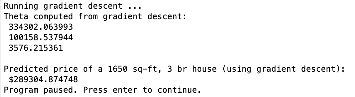
用梯度下降选择参数theta并且预测
这段代码包含于主函数代码中1
2
3
4
5
6
7
8
9
10
11
12
13
14
15
16
17
18
19
20
21
22
23
24
25
26
27
28
29
30
31
32
33
34
35
36
37
38fprintf('Running gradient descent ...\n');
% Choose some alpha value
alpha = 0.01;
num_iters = 400;
% Init Theta and Run Gradient Descent
theta = zeros(3, 1);
[theta, J_history] = gradientDescentMulti(X, y, theta, alpha, num_iters);
% Plot the convergence graph
figure;
plot(1:numel(J_history), J_history, '-b', 'LineWidth', 2);
xlabel('Number of iterations');
ylabel('Cost J');
% Display gradient descent's result
fprintf('Theta computed from gradient descent: \n');
fprintf(' %f \n', theta);
fprintf('\n');
% Estimate the price of a 1650 sq-ft, 3 br house
% ====================== YOUR CODE HERE ======================
% Recall that the first column of X is all-ones. Thus, it does
% not need to be normalized.
%price = 0; % You should change this
x = [1650 3];
x = (x - mu) ./ sigma;
x = [ones(1, 1) x];
price = x * theta;
% ============================================================
fprintf(['Predicted price of a 1650 sq-ft, 3 br house ' ...
'(using gradient descent):\n $%f\n'], price);
fprintf('Program paused. Press enter to continue.\n');
pause;
运行结果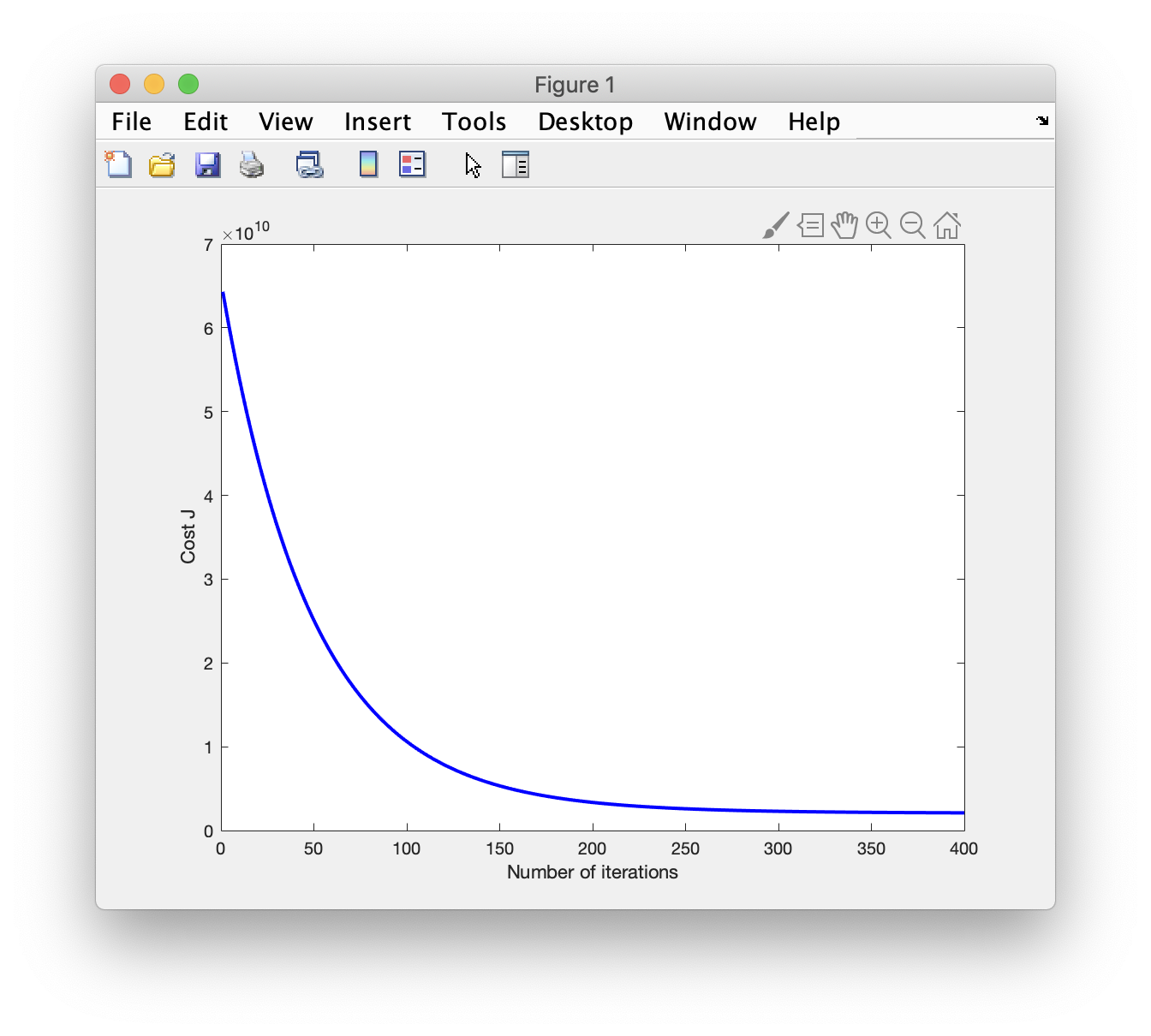
Part 3: Normal Equations
正规方程
非迭代方法选择参数,并做与上述相同的预测
normalEqn.m1
2
3
4
5
6
7
8
9
10
11
12
13
14
15
16function [theta] = normalEqn(X, y)
%NORMALEQN Computes the closed-form solution to linear regression
% NORMALEQN(X,y) computes the closed-form solution to linear
% regression using the normal equations.
theta = zeros(size(X, 2), 1);
% ====================== YOUR CODE HERE ======================
% Instructions: Complete the code to compute the closed form solution
% to linear regression and put the result in theta.
%
theta = pinv(X'*X)*X'*y;
% ============================================================
end
运行结果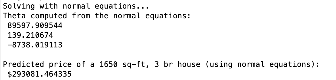
主函数代码
ex1_multi.m1
2
3
4
5
6
7
8
9
10
11
12
13
14
15
16
17
18
19
20
21
22
23
24
25
26
27
28
29
30
31
32
33
34
35
36
37
38
39
40
41
42
43
44
45
46
47
48
49
50
51
52
53
54
55
56
57
58
59
60
61
62
63
64
65
66
67
68
69
70
71
72
73
74
75
76
77
78
79
80
81
82
83
84
85
86
87
88
89
90
91
92
93
94
95
96
97
98
99
100
101
102
103
104
105
106
107
108
109
110
111
112
113
114
115
116
117
118
119
120
121
122
123
124
125
126
127
128
129
130
131
132
133
134
135
136
137
138
139
140
141
142
143
144
145
146
147
148
149
150
151
152
153
154
155
156
157
158
159
160
161
162%% Machine Learning Online Class
% Exercise 1: Linear regression with multiple variables
%
% Instructions
% ------------
%
% This file contains code that helps you get started on the
% linear regression exercise.
%
% You will need to complete the following functions in this
% exericse:
%
% warmUpExercise.m
% plotData.m
% gradientDescent.m
% computeCost.m
% gradientDescentMulti.m
% computeCostMulti.m
% featureNormalize.m
% normalEqn.m
%
% For this part of the exercise, you will need to change some
% parts of the code below for various experiments (e.g., changing
% learning rates).
%
%% Initialization
%% ================ Part 1: Feature Normalization ================
%% Clear and Close Figures
clear ; close all; clc
fprintf('Loading data ...\n');
%% Load Data
data = load('ex1data2.txt');
X = data(:, 1:2);
y = data(:, 3);
m = length(y);
% Print out some data points
fprintf('First 10 examples from the dataset: \n');
fprintf(' x = [%.0f %.0f], y = %.0f \n', [X(1:10,:) y(1:10,:)]');
fprintf('Program paused. Press enter to continue.\n');
pause;
% Scale features and set them to zero mean
fprintf('Normalizing Features ...\n');
[X, mu, sigma] = featureNormalize(X);
% Add intercept term to X
X = [ones(m, 1) X];
%% ================ Part 2: Gradient Descent ================
% ====================== YOUR CODE HERE ======================
% Instructions: We have provided you with the following starter
% code that runs gradient descent with a particular
% learning rate (alpha).
%
% Your task is to first make sure that your functions -
% computeCost and gradientDescent already work with
% this starter code and support multiple variables.
%
% After that, try running gradient descent with
% different values of alpha and see which one gives
% you the best result.
%
% Finally, you should complete the code at the end
% to predict the price of a 1650 sq-ft, 3 br house.
%
% Hint: By using the 'hold on' command, you can plot multiple
% graphs on the same figure.
%
% Hint: At prediction, make sure you do the same feature normalization.
%
fprintf('Running gradient descent ...\n');

% Choose some alpha value
alpha = 0.01;
num_iters = 400;

% Init Theta and Run Gradient Descent
theta = zeros(3, 1);
[theta, J_history] = gradientDescentMulti(X, y, theta, alpha, num_iters);

% Plot the convergence graph
figure;
plot(1:numel(J_history), J_history, '-b', 'LineWidth', 2);
xlabel('Number of iterations');
ylabel('Cost J');

% Display gradient descent's result
fprintf('Theta computed from gradient descent: \n');
fprintf(' %f \n', theta);
fprintf('\n');

% Estimate the price of a 1650 sq-ft, 3 br house
% ====================== YOUR CODE HERE ======================
% Recall that the first column of X is all-ones. Thus, it does
% not need to be normalized.
%price = 0; % You should change this
x = [1650 3];
x = (x - mu) ./ sigma;
x = [ones(1, 1) x];
price = x * theta;

% ============================================================

fprintf(['Predicted price of a 1650 sq-ft, 3 br house ' ...
         '(using gradient descent):\n $%f\n'], price);

fprintf('Program paused. Press enter to continue.\n');
pause;
%% ================ Part 3: Normal Equations ================
fprintf('Solving with normal equations...\n');
% ====================== YOUR CODE HERE ======================
% Instructions: The following code computes the closed form
% solution for linear regression using the normal
% equations. You should complete the code in
% normalEqn.m
%
% After doing so, you should complete this code
% to predict the price of a 1650 sq-ft, 3 br house.
%
%% Load Data
data = csvread('ex1data2.txt');
X = data(:, 1:2);
y = data(:, 3);
m = length(y);
% Add intercept term to X
X = [ones(m, 1) X];
% Calculate the parameters from the normal equation
theta = normalEqn(X, y);
% Display normal equation's result
fprintf('Theta computed from the normal equations: \n');
fprintf(' %f \n', theta);
fprintf('\n');
% Estimate the price of a 1650 sq-ft, 3 br house
% ====================== YOUR CODE HERE ======================
%price = 0; % You should change this
x = [1650 3];
x = [ones(1, 1) x];
price = x * theta;
% ============================================================
fprintf(['Predicted price of a 1650 sq-ft, 3 br house ' ...
'(using normal equations):\n $%f\n'], price);
实验一完成